This page provides an introduction to CAT from Prof. David J. Weiss at the University of Minnesota.

Computerized adaptive testing (CAT) is the redesign of psychological and educational measuring instruments for delivery by interactive computers. CAT can be used for tests of ability or achievement and for measures of personality and attitudinal variables. Its objective is to select, for each examinee, the set of test questions from a pre-calibrated item bank that simultaneously most effectively and efficiently measures that person on the trait.

This section focuses on CAT that uses item response theory (IRT) as the psychometric model. Not all approaches to CAT use IRT. When a test is being used to classify an examinee, the problem can be approached from an IRT perspective or from a decision theory perspective. For example, Lawrence Rudner has proposed a measurement decision theory (MDT) approach to making mastery or other dichotomous classification decisions. His MDT Web site describes how this approach works and provides an interactive tutorial on MDT, as well as other resources and references on MDT and related issues.

IThe basic principle of adapting a test to each examinee was recognized in the very early days of psychological measurement, even before the development of the standardized conventional paper-and-pencil test, by Alfred Binet in the development of the Binet IQ test (Binet & Simon, 1905) which later was published as the Stanford-Binet IQ Test. Binet’s test was comprised of sets of test items normed by chronological age level.

Binet’s test administration procedure is a fully adaptive procedure (see example below):

1. It uses a pre-calibrated bank of test items. Binet selected items for each age level if approximately 50% of the children at that age level answered an item correctly. Thus, in the original version of the test, there were sets of items at ages from three years through 11 years. All of these items constituted “Binet’s item bank” for his adaptive test.

2. It is individually administered by a trained psychologist and is designed to “probe” for the level of difficulty (i.e., chronological age) that is most appropriate for each examinee, much as hurdle-jumping probes for the performance level of each athlete.

3. It has a variable starting option. The Binet test is begun by the administrator based on her/his best guess about the examinee’s likely ability level (typically the examinee’s chronological age, but it can be lower or higher if there is information to inform such a starting level).

4. It use a defined scoring method – a set of items at a given age level is administered and immediately scored by the administrator.

5. There is a “branching” or item selection rule that determines which items will next be administered to a given examinee. In the Binet test, the next set of items to be administered is based on the examinee’s performance on each previous set of items. If the examinee has answered some or most of the items at a given age level correctly, usually the items at the next higher age level are administered. If most of the items at a given age level are answered incorrectly, items at the next lower age level are typically administered.

6. There is a pre-defined termination rule. The Binet test is terminated when, for each examinee, both a “ceiling” and a “basal” level have been identified. The ceiling level is the age level at which the examinee incorrectly answers all items; the basal level is the age level at which the examinee correctly answers all the items. The effective range of measurement for each examinee lies between these two levels.

An examinee’s final score on the Binet test is based on the subset of items that she/he answered correctly. In effect, these items are weighted by their age level in arriving at the IQ scores derived from the test, since different examinees will answer both different numbers and subsets of items.

In 1973 I proposed a variation of the Binet test that required a computer for administration (Weiss, 1973) in an attempt to make the test more efficient. I called it the “stratified adaptive” or “stradaptive” test.

The stradaptive test uses the same item bank structure as the Binet test. That is, test items are stratified or organized into levels of difficulty, referred to as “strata.” Similar to the Binet test,it uses a variable starting level that allows the test to begin at any level of difficulty deemed appropriate for each examinee. The stradaptive test procedure differs from the Binet test, however, in its “branching” rule and in its termination rule.

In the Binet test, a set of items at a given difficulty level (stratum) is administered and scored. Based on the examinee’s score on that set of items, the examiner selects either a more difficult or a less difficult stratum for the next set of items, In the stradaptive test, a single item is administered and scored. A branching decision is then made after each item. If the item was answered correctly, the first unadminstered item in the next more difficult stratum is administered. If the item was answered incorrectly, the first unadministered item in the next less difficult stratum is administered. This process of scoring an item and branching up or down in difficulty depending on the item score is continuedon an item-by-item basis until a termination criterion is reached.

A Binet test is terminated when both a ceiling level and a basal level are identified for each examinee. The ceiling level is that stratum at which all items were answered incorrectly; the basal level is the stratum at which all items are answered incorrectly. The stradaptive test termination criterion uses only a variation of the ceiling level. The stradaptive test can be termination when all items at any level are answered incorrectly (i.e., Binet’s ceiling level) or string of five consecutive items in a given stratum are incorrectly answered.

An Example Stradaptive Test

Figure 1 shows a sample response record from a stradaptive test. In this figure, a “+” indicates a correct answer to a test question and a “-” indicates an incorrect response. Items are “stratified” into “Mental Age” levels (as they are in a Binet-type test), with 10 items at each level. The two columns on the right show the number of items administered at each Mental Age stratum and the proportion correct at that stratum.

Figure 1. A Sample Stradaptive Test Response Record

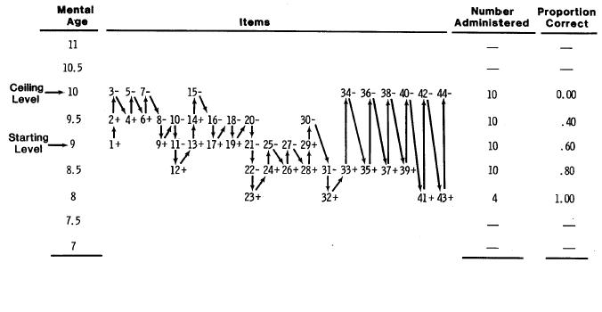
The stradaptive test permits a variable starting level. In this test, the starting level was Mental Age 9. The first item (1) was administered and answered correctly (+), so the next item administered was the first unadministered item at Age 9.5. This item was answered correctly, so the first item at Age 10 was administered (Item 3). This item was answered incorrectly (3-), so the next available item at the next lower stratum (Age 9.5) was administered and answered correctly (4+).

The process of administering an item, scoring item, and branching up or down depending on whether the item was answered correctly continued through Item 30. Item 30 was answered incorrectly, but all 10 items at Age 9 had been administered So the next item administered was the sixth available item at Age 8.5. One-stratum branching then continued for Items 31-33. But because all 10 items at Age 9 had been administered, three-stratum branching began after Item 33 was answered correctly. Finally, after all items at Age 8.5 were used, four-stratum branching was used for Items 40 to 44.

The stradaptive test was terminated when a “ceiling level” had been identified. The ceiling level is determined when all items at a given stratum were incorrectly answered. This occurred when Item 44 was incorrectly answered (44-), resulting in incorrect answers to all items at Mental Age 10.

The Proportion Correct column shows the typical results of a stradaptive test. As expected, the proportion correct increases (from 0.0 to 1.0) as the item difficulty (Mental Age) decreases. In addition, the overall proportion correct is at the optimal level of .50.

Reference

Weiss, D. J. (1973). The stratified adaptive computerized ability test (Research Report 73-3). Minneapolis: University of Minnesota, Department of Psychology, Psychometric Methods Program, Computerized Adaptive Testing Laboratory.

IRT is a family of mathematical models that describe how people interact with test items (Embretson & Reise, 2000). These models were originally developed for test items that are scored dichotomously (correct or incorrect) but the concepts and methods of IRT extend to a wide variety of polytomous models for all types of psychological variables that are measured by rating scales of various kinds (Van der Linden & Hambleton, 1997). Additional resources on IRT.

In the context of items scored correct/incorrect, test items are described by their characteristics of difficulty and discrimination, as they are in traditional item and test analysis. But in IRT, these item statistics (referred to as “parameters”) are estimated and interpreted differently than classical proportion correct and item-total correlation. For multiple-choice items, IRT adds a third item parameter referred to as a “pseudo-guessing” parameter that reflects the probability that an examinee with a very low trait level will correctly answer an item solely by guessing.

Information

Although these three item parameters are useful in their own right, for purposes of CAT they are combined into an “item information function” (IIF). The IIF is computed from the item parameters. It describes how well, or precisely, an item measures at each level of the trait that is being measured by a given test (referred to in IRT by the Greek letter theta). A major advantage of IRT is that both items and people are placed on the same scale (usually a standard score scale, with mean = 0.0, and standard deviation = 1.0) so that people can be compared to items and vice-versa.

Figure 1 shows IIFs for 10 items. The location of the center of the IIF reflects the difficulty of the item, the height of the IIF reflects the item discrimination, and its asymmetry reflects the magnitude of the pseudo-guessing parameter. Thus, because Item 1 is the easiest item its IIF is on the left end of the theta continuum, and Item 10 is the most difficult. Because Item 9 is the most discriminating it has the highest IIF, and Item 7 is the least discriminating. None of these items has a high pseudo-guessing parameter since all of the IIFs are reasonably symmetric.

Figure 1
Information Functions for 10 Items

IRT Scoring: Maximum Likelihood Estimation

Whereas tests not using IRT are typically scored by number correct, or if using rating scale items by summing a set of arbitrary weights, IRT uses a quite different method of scoring or estimating theta levels for examinees. This method is called “maximum likelihood estimation” (MLE). In contrast to number-correct scoring, MLE weights each item by all three of its item parameters and also considers whether the examinee answered each item correctly. As a result of combining information on the examinee’s entire pattern of responses as well as the characteristics of each item, MLE can provide many more distinctions among examinees than can number-correct scoring. For example, number-correct scoring of a 10-item conventional test can result in at most 11 scores (0 to 10); MLE for the same test can result in 1,024 (2 raised to the 10th power) different theta estimates.

MLE has an additional advantage over number-correct scoring. In addition to providing a for each examinee, MLE also provides an individualized standard error of measurement (SEM) for each. Unlike the SEMs from non-IRT test analysis methods, the SEMs from IRT can vary from person to person, depending on how they answered a particular set of items. Finally, the theta estimates and their SEMs in IRT are not dependent on a particular set of items – they can be determined from any subset of items that an examinee has taken, as long as the parameters for those items have been estimated on the same scale.

References

Embretson, S. E. & Reise, S. P. (2000). Item response theory for psychologists. Mahwah NJ, Lawrence Erlbaum Associates.
Van der Linden, W. J. & Hambleton, R. K. (1997). Handbook of item response theory. New York, Springer-Verlag.

In IRT-based CAT, a relatively large item bank is developed for a given trait and their item information functions are determined. A good CAT item bank has items that collectively provide information across the full range of the trait (theta). An examinee begins the CAT with an initial theta estimate, which can be the same for all examinees, or can use any prior information available on the examinee (e.g., performance on other tests, grade level, information from teachers). An item is administered based on that initial theta estimate and immediately scored by the computer that is delivering the test.

Item Selection

IRT-based CAT selects each next item based on the examinee’s scored responses to all previous items. At the initial stages of a CAT, when only a single item or two has been administered, the next item is usually selected by a “step” rule – if the first item was answered correctly, the examinee’s original prior theta estimate is increased by some amount (e.g., .50); if the first item was answered incorrectly, the original theta estimate is decreased by the same amount. As the test proceeds and the examinee obtains a response pattern of at least one correct and one incorrect response,maximum likelihood estimation (MLE) is used to obtain a new theta estimate, which is based on the examinee’s responses to all administered items at that point in the test.

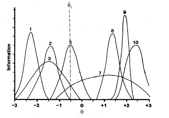
After each item is administered and scored, the new theta estimate is used to select the next item. That item is the unadministered item in the item bank that provides the most information at the current theta estimate. Figure 1 – 3 illustrate “maximum information” item selection in CAT. In addition to displaying information functions for 10 items, Figure 1 shows an initial theta estimate for a hypothetical examinee (indicated by the vertical line). This value is shown at 0.0, which is the mean of the theta scale. Values of information are computed for all items at that theta level. Figure 1 shows that Item 6 provides the most information of the 10 items at theta = 0.0. Therefore, Item 6 is administered and scored.Figure 1
Information Functions for 10 Items

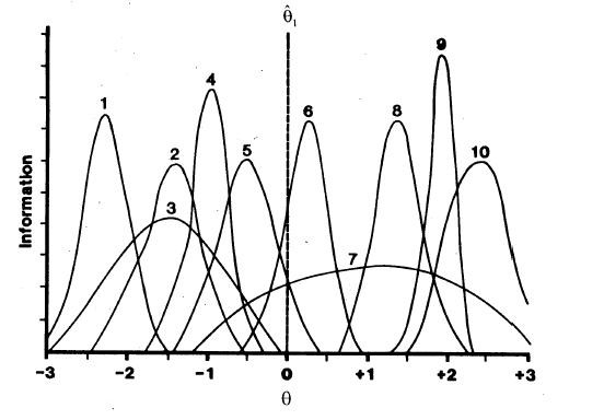
Based on that score (incorrect, in this example), a new theta estimate is determined (in this case using a step size of 1.0) as –1.0. Based on the maximum information item selection rule, Item 4 is administered (Figure 2), because it is the item at that theta level that has maximum information,and scored. Assuming that Item 4 was answered correctly, MLE can now be used to estimate theta.

Figure 2
Information Functions for 9 Items

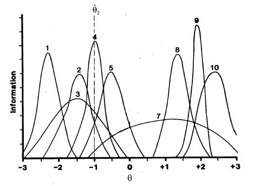
The result is theta = -.50. Again,selecting an item by maximum information results in the selection of Item 5 (Figure 3). Scoring, theta estimation, and item selection continue until a termination criterion is reached.Figure 3
Information Functions for 8 Items

Ending a CAT

One important characteristic of CAT is that the test termination criterion can be varied for different testing objectives. Some tests are used for selection or classification, for example to classify an individual as having mastered some domain of achievement or to select those who will be admitted to a school or college or hired for a job. Other tests are used for counseling or clinical purposes. The objective of such tests is to measure each individual as well as possible. In the context of CAT, these two objectives are operationalized by two different termination rules.For classification purposes, an individual’s score is compared against some cutoff value. The objective is to make as accurate a classification as possible. To implement this in the context of CAT, both the theta estimate and its associated SEM are used. An individual can be classified as being above a cutoff value (expressed on the theta scale) if both the theta estimate and its 95% confidence interval (calculated as plus or minus two SEMs) are above or below the cut score. Since CAT can evaluate this decision after each item is administered, the test can be terminated when this condition is satisfied. The result of such a test will be a set of classifications made for a group of examinees that all have at most a 5% error rate. The error rate can be controlled by changing the size of the SEM confidence interval around the theta estimate.

When CATs are not used for classification, a different termination rule applies. In this case, it is desirable to measure each examinee to a desired level of precision, as determined by a predetermined level of SEM. This will result in a set of “equiprecise” measurements, such that all examinees will have scores that are equivalently accurate – perhaps defining a new concept of “test fairness.” To implement equiprecise measurement, CAT allows the user to specify the level of SEM that is desired for each examinee. Assuming that the item bank has a sufficient number of test items properly distributed across the theta scale and the test is allowed to continue long enough for examinee, this goal will be achieved if the test is terminated when that level of SEM is reached.

A Sample CAT Report

Figure 4 shows the response record of a single examinee’s progress through a CAT. This CAT was designed to make a dichotomous classification around theta = 1.0 (1 standard deviation above the mean), with a plus or minus 1 standard error of measurement (SEM) band (a 68% confidence interval). The initial theta estimate (X) was 0.0 and the test item providing maximum information at that theta level was administered and answered correctly (C). The initial step size was 3.0 to attempt to force a mixed correct/incorrect) response pattern as quickly as possible, so the next item had maximum information at theta = 3.0. It, too, was answered correctly so additional difficult questions were given (Items 3 and 4) until an incorrect answer (I) was obtained. At that point, maximum likelihood estimation was used to obtain a theta estimate of 2.66. The item at that level (Item 5) was also answered incorrectly and the resulting theta estimate 1.87 with an SEM of .94. Note that each time a correct answer was obtained, the theta estimate increased, and an incorrect answer led to a decrease in estimated theta. Note also that the differences between successive estimated thetas decreased as the test proceeded, indicating that the test was converging on the examinee’s theta level; also, in general, the SEM tended to decrease, since additional item responses generally improve the estimation of theta.

In this test, the examinee’s estimated theta followed a downward trend, falling below the cut score of theta = 1.0 at Item 15. But the estimated theta could not be assumed to be reliably below that cut score because the SEM band still included theta = 1.0. So the test continued for another 10 items until the examinee’s estimated theta and its SEM were entirely below the cut score. This occurred at Item 20 (.55 + .43 = .98, which is just below 1.00) and the test was terminated. The test results indicate that this examinee’s estimated theta was below the cut score, with at least 68% confidence (actually, in this case because that confidence interval was symmetric and 50% was below the mean, the confidence level of a unidirectional decision would be 50% + 34% = 84%). Higher confidence could have been obtained by using a 2 SEM interval around estimated theta, which obviously would have a required a longer test.Figure 4
Item-By-Item Report of a Maximum Information CAT for a Single Examinee

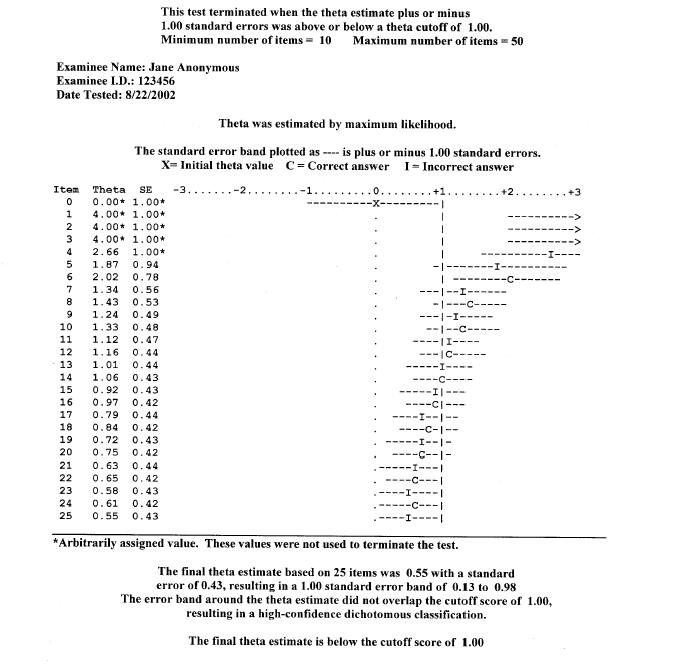
Figure 4 also illustrates another characteristic of most CATs: As the test progresses, the examinee tends to alternate between correct and incorrect answers, as can be seen beginning with Item 7 or 8. This is the result of the convergence process that underlies CAT. The result, typically, is that each examinee will answer a set of questions on which he/she obtains 50% correct, even though each examinee will likely receive a set of questions of differing difficulty. In a sense, this characteristic of a CAT tends to equalize the #8220;psychological environment” of the test across examinees of different trait levels. By contrast, in a conventional test the examinee who is high on the trait will answer most items correctly and the low trait examinee will answer most of the items incorrectly.

Although this example is a CAT designed to make a dichotomous classification, the same principles would be observed in a CAT designed to measure each examinee to a prespecified level of precision (an “equiprecise “CAT). The only difference would be in the termination criterion. Rather than ending the CAT when the theta estimate was reliably below the cut score, an equiprecise CAT would end when the SEM associated with the theta estimate fell below a prespecified value (e.g., .20).